Can a Baby Learn? A Toy Model of Discipline and Desire
Part I: Q-learning
I’m a father of two, and raising my kids gives me a lot of joy. I love teaching them and seeing them learn, whether from me or on their own. Lately, I have been contemplating how important consistency and patience are when teaching my kids.
More often than not, kids will not listen to you. This is just how it is. For a two-year-old, that colourful remote control is just too inviting. Climbing a chair is just one adventure that one cannot refuse, and so on. The mighty “No!” is not enough.
After a while, the “No” slowly starts to work. Babies learn at their own pace, but what intrigues me is why some learn, and others don’t. Of course, there might be an innate reason, but I doubt anyone would question that the environment and the caretaker play a big role.
One big thing I’ve always noticed is consistency. It is always important for the caretakers to be consistent with the rules at home. No is No. Something else is that harsh treatment (yelling, spanking) clearly has negative effects on the kid. I keep these two ideas in mind whenever I’m working with any learning human, not just my kids.
Thinking about this, I decided to see whether I could model it in a learning agent. The idea is simple: I want to model an agent whose learning is shaped by two things: i) caretaker consistency (how stable the payoff is) and ii) harsh treatment (punishment beyond the normal “No”).
Before anything, a disclaimer. This is just a simple model. I can promise you no brain works like the models I’ll show in this and the next part. This is just an exercise.
The child
Take a little girl too young to climb a chair on her own. To her, climbing looks fun: she puts an inner fun value $v_{fun} = 10$ on it. Her father has other plans. He wants to discourage the climbing, so every time she tries, he says “No” and blocks her. The “No” isn’t free for her: it carries a cost penalty $c_{penalty} = 20$. So the reward $r_t$ she experiences on attempt $t$ is:
$$r_t = \begin{cases} v_{fun} = 10 & \text{the father lets her climb}, \\[2pt] v_{fun} - c_{penalty} = -10 & \text{the father says ``No''}. \end{cases}$$Notice that a blocked attempt is a net negative even though climbing is fun: $10 - 20 = -10$.
She doesn’t take one experience at face value. She keeps a running estimate $Q_t$ of what climbing is worth, and after each attempt she moves that estimate a fraction $\alpha$ toward the reward she just received. This is the simplest model in reinforcement learning: a Q-value updated by a prediction error. Economists will recognise it as adaptive expectations:
$$Q_{t+1} = Q_t + \alpha\, (r_t - Q_t),$$where $r_t - Q_t$ is her surprise: how much the experience differed from what she expected. Repeatedly, $Q_t$ settles on the value of the payoff the father actually delivers.
1. Consistent vs. Inconsistent Father
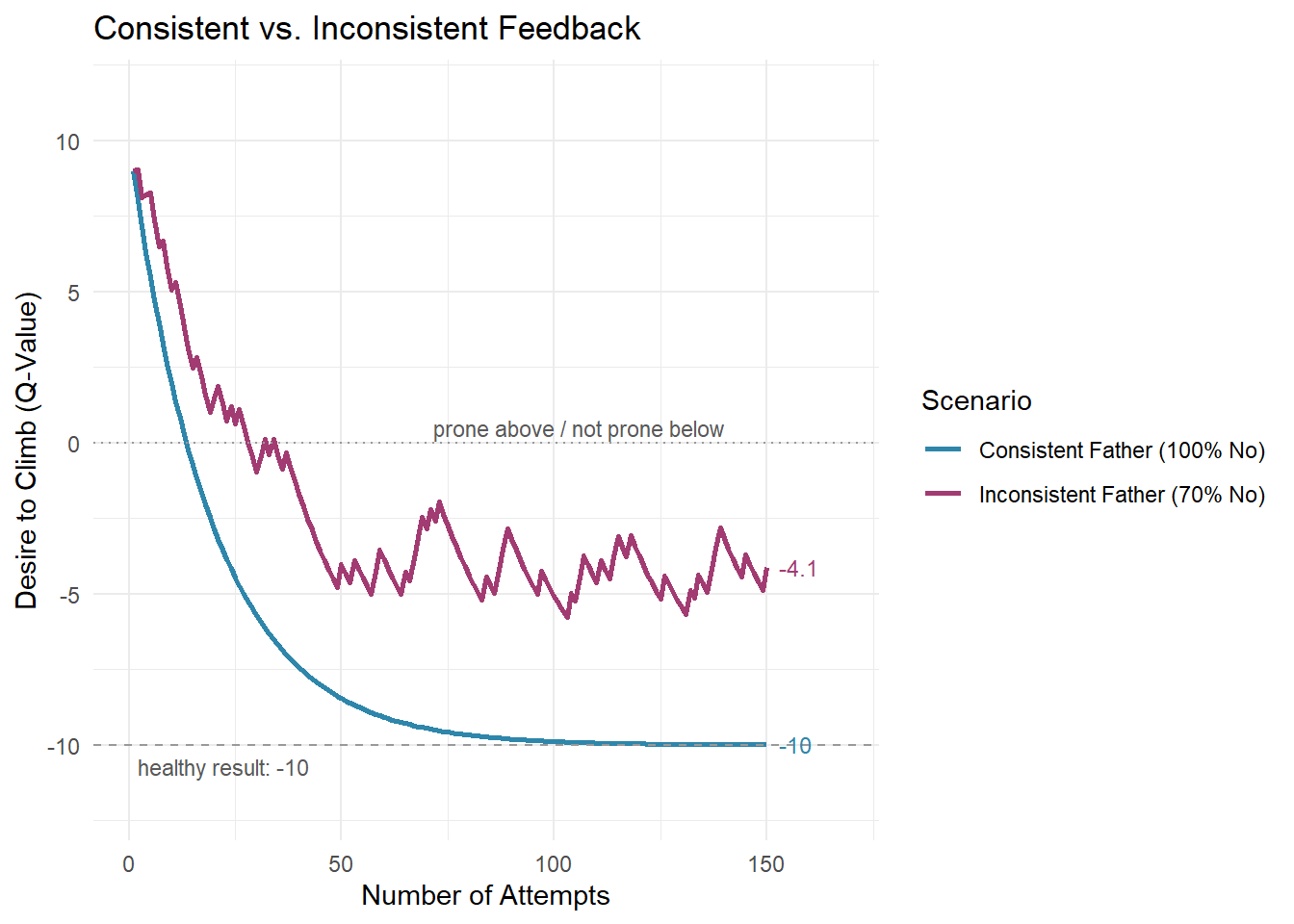
Now consider two types of father: a consistent one and an inconsistent one who says no with probability $\gamma = 70\%$.
$$r_t = \begin{cases} v_{fun} - c_{penalty} & \text{with probability } \gamma, \\[2pt] v_{fun} & \text{with probability } 1 - \gamma, \end{cases}$$so the Q-value converges to the expected payoff $10 \cdot 0.3 - 10 \cdot 0.7 = -4$, and it keeps wobbling because the signal is noisy:
$$\mathbb{E}[r_t] = v_{fun} - \gamma\, c_{penalty} = -4$$The dashed line marks this healthy result. The consistent child lands exactly on $-10$. Values above 0 mean the child is still prone to climb the chair.
Why is $-10$ the “healthy” line? Because it is the honest price of the chair: $+10$ of fun, blocked for $20$, so $-10$ is the desire that matches reality. This says nothing about what sits between the zones. The model only moves the desire. A child drifting only slightly off $-10$ may follow the rule while quietly questioning the father, while a child far from it (far below, from harsh punishment, or clearly positive, from inconsistency) may be closer to fear or trauma than to learning. We do not model those zones. The distance from $-10$ is left for the reader to judge.
Below is the code that generates a simulation for each type of father.
library(ggplot2)
library(dplyr)
library(tidyr)

simulate_learning <- function(
    trials = 150,
    learning_rate = 0.05,
    v_fun = 10,
    c_penalty = 20,
    gamma_inconsistent = 0.7,
    initial_q = 10
) {
  results <- data.frame(
    trial = 1:trials,
    q_consistent = numeric(trials),
    q_inconsistent = numeric(trials)
  )
  q_c <- q_i <- initial_q
  for (t in 1:trials) {
    reward_c <- v_fun - c_penalty
    q_c <- q_c + learning_rate * (reward_c - q_c)
    reward_i <- ifelse(runif(1) < gamma_inconsistent, v_fun - c_penalty, v_fun)
    q_i <- q_i + learning_rate * (reward_i - q_i)
    results$q_consistent[t] <- q_c
    results$q_inconsistent[t] <- q_i
  }
  return(results)
}

set.seed(123)
data <- simulate_learning()

data_long <- data %>%
  pivot_longer(cols = starts_with("q_"), names_to = "Father_Type", values_to = "Q_Value")

ggplot(data_long, aes(x = trial, y = Q_Value, color = Father_Type)) +
  geom_line(linewidth = 1) +
  geom_hline(yintercept = -10, linetype = "dashed", color = "grey60") +
  geom_hline(yintercept = 0, linetype = "dotted", color = "grey60") +
  annotate("text", x = 2, y = -10.7, label = "healthy result: -10", hjust = 0, color = "grey35", size = 3) +
  annotate("text", x = 140, y = 0.5, label = "prone above / not prone below", hjust = 1, color = "grey35", size = 3) +
  geom_text(data = data_long %>% group_by(Father_Type) %>% slice_tail(n = 1),
            aes(x = 153, label = round(Q_Value, 1)), hjust = 0, size = 3.2, show.legend = FALSE) +
  scale_x_continuous(limits = c(0, 168)) +
  scale_y_continuous(limits = c(-12, 11.5)) +
  scale_color_manual(
    values = c("q_consistent" = "#2E86AB", "q_inconsistent" = "#A23B72"),
    labels = c("Consistent Father (100% No)", "Inconsistent Father (70% No)")
  ) +
  labs(
    title = "Consistent vs. Inconsistent Feedback",
    x = "Number of Attempts",
    y = "Desire to Climb (Q-Value)",
    color = "Scenario"
  ) +
  theme_minimal()
2. Adding Harsh Punishment
Now consider a father who loses his temper and says “No” harshly with probability $\varepsilon$. Severe repression has a $s$ multiplier effect on the $c_{penalty}$.
$$r_t = \begin{cases} v_{fun} - s\, c_{penalty} & \text{with probability } \varepsilon \text{ (harsh ``No'')},\\[2pt] v_{fun} - c_{penalty} & \text{otherwise}. \end{cases}$$For comparison, assume a father who always yields, one who consistently says no, one who gives a harsh “no” ($\varepsilon = 0.02$), and an inconsistent one ($\gamma = 0.7$).
simulate_four_scenarios <- function(
    trials = 200,
    learning_rate = 0.08,
    gamma_inconsistent = 0.7,
    v_fun = 10,
    c_penalty = 20,
    harsh_prob = 0.02
) {
  q <- c(consist = 10, always = 10, incons = 10, harsh = 10)
  history <- data.frame()
  for (t in 1:trials) {
    r_consist <- v_fun - c_penalty
    q["consist"] <- q["consist"] + learning_rate * (r_consist - q["consist"])
    r_always <- v_fun
    q["always"] <- q["always"] + learning_rate * (r_always - q["always"])
    r_incons <- ifelse(runif(1) < gamma_inconsistent, v_fun - c_penalty, v_fun)
    q["incons"] <- q["incons"] + learning_rate * (r_incons - q["incons"])
    harsh_shock <- ifelse(runif(1) < harsh_prob, 1, 0)
    r_harsh <- ifelse(harsh_shock == 1, v_fun - 3 * c_penalty, v_fun - c_penalty)
    q["harsh"] <- q["harsh"] + learning_rate * (r_harsh - q["harsh"])
    history <- rbind(history, data.frame(
      trial = t,
      Consistent = q["consist"],
      Always_Yields = q["always"],
      Purely_Inconsistent = q["incons"],
      Harsh_punishment = q["harsh"],
      harsh_shock = harsh_shock
    ))
  }
  return(history)
}

set.seed(789)
results <- simulate_four_scenarios()

results_long <- results %>%
  select(-harsh_shock) %>%
  pivot_longer(-trial, names_to = "Father_Type", values_to = "Desire")

ggplot(results_long, aes(x = trial, y = Desire, color = Father_Type)) +
  geom_line(linewidth = 1) +
  geom_hline(yintercept = -10, linetype = "dashed", color = "grey60") +
  geom_hline(yintercept = 0, linetype = "dotted", color = "grey60") +
  annotate("text", x = 2, y = -10.7, label = "healthy result: -10", hjust = 0, color = "grey35", size = 3) +
  annotate("text", x = 190, y = 0.5, label = "prone above / not prone below", hjust = 1, color = "grey35", size = 3) +
  geom_text(data = results_long %>% group_by(Father_Type) %>% slice_tail(n = 1),
            aes(x = 203, label = round(Desire, 1)), hjust = 0, size = 3.2, show.legend = FALSE) +
  scale_x_continuous(limits = c(0, 218)) +
  scale_y_continuous(limits = c(-15, 11.5)) +
  scale_color_manual(values = c(
    "Always_Yields" = "#2ECC71",
    "Consistent" = "#E74C3C",
    "Purely_Inconsistent" = "#9B59B6",
    "Harsh_punishment" = "#BBB111"
  )) +
  labs(
    title = "Four Parenting Styles",
    x = "Attempts",
    y = "Expected Utility (Q-Value)",
    color = "Scenario"
  ) +
  theme_minimal()
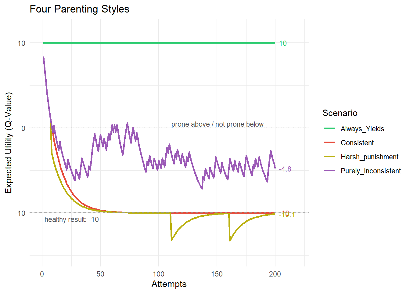
The expected payoff shifts only slightly, $\mathbb{E}[r_t] = v_{fun} - c_{penalty} - \varepsilon\,(s - 1)\, c_{penalty} = -10.8$. And the harsh child learns at the same step size as everyone else ($\alpha = 0.08$): the learning rate is the same. An early harsh event can still speed up the initial descent. The surprise is much bigger, and one shock drops the Q-value several points at once (here it lands at attempt 8, putting her about 5 attempts ahead of the consistent child). What harshness does not change is the pace of convergence: the curve settles toward its target at the same speed, just below it. Harshness does not speed up the lesson; it bends the target: the child settles slightly below the healthy -10 line.
A side note: harshness can buy consistency. In this model, harsh treatment has no consequences. No state builds up; nothing carries over. Under that assumption, an inconsistent father can compensate: the expected payoff only depends on the effective “No” rate $\gamma + \varepsilon\,(s - 1)$. A father who lets the child climb 70% of the time ($\gamma = 0.3$) can still bring the desire to the healthy $-10$ by punishing harshly in $\varepsilon = 0.35$ of attempts, since $0.3 + 2 \cdot 0.35 = 1$. The catch is that this works only on average. The shocks keep pulling the Q-value around, and it stops working the moment harshness has consequences, as the next section shows.
3. Too Much Harsh Punishment: A State-Space View
Now harshness is no longer just a rare event. It becomes a condition the child internalises.
The learning rate is no longer a fixed constant either: it becomes state-dependent, a function of the hidden state the child carries. In machine-learning terms, this is the child learning to learn: plasticity itself becomes a function of experience.
Each harsh event $e_t$, a coin flip with probability $\varepsilon$, adds to a hidden state $h_t$: her accumulated harshness exposure. The state decays slowly, at rate $\varphi$ (phi = 0.99):
The state eats into learning. The more exposure, the smaller the step size (a frightened child updates less and less), floored at $\alpha_{min}$:
$$\alpha_t = \max\!\left( \frac{\alpha_0}{1 + \beta\, h_t},\ \alpha_{min} \right),$$with $\beta = 10$ and $\alpha_0 = 0.1$. The payoff keeps the previous form, now tied to the event:
$$Q_{t+1} = Q_t + \alpha_t\, (r_t - Q_t), \qquad r_t = \begin{cases} v_{fun} - s\, c_{penalty} & \text{if } e_t = 1,\\[2pt] v_{fun} - c_{penalty} & \text{if } e_t = 0. \end{cases}$$The timing matters: the update on attempt $t$ uses the step size the child carried before the event, so a harsh look lands at full strength; the whole sting registers. The suppressed step size then governs everything that follows, which is why each shock bites once and then leaves the child slow to learn until the state decays back.
Below are three scenarios: no harsh events, 1% harsh events, and 60% harsh events. With no severe events, the step size stays at its baseline $\alpha_{0} = 0.1$. With 1%, the state pops up after each rare shock, and the learning rate dips until it decays back. With 60%, the state saturates, and the step size collapses.
simulate_harsh_state_space <- function(
    trials = 200,
    lr0 = 0.1,
    v_fun = 10,
    c_penalty = 20,
    initial_q = 10,
    harsh_prob = 0.01,
    harsh_severity = 3,
    phi = 0.99,
    beta = 10,
    lr_floor = 0.0005
) {
  h <- 0
  q <- initial_q
  lr <- lr0
  history <- data.frame()
  for (t in 1:trials) {
    harsh_event <- ifelse(runif(1) < harsh_prob, 1, 0)
    reward <- ifelse(harsh_event == 1, v_fun - harsh_severity * c_penalty, v_fun - c_penalty)
    q <- q + lr * (reward - q)
    h <- phi * h + harsh_event
    lr <- max(lr0 / (1 + beta * h), lr_floor)
    history <- rbind(history, data.frame(trial = t, h = h, lr = lr, q = q))
  }
  return(history)
}

set.seed(42)
never_harsh <- simulate_harsh_state_space(harsh_prob = 0.00, harsh_severity = 3)
occasional_harsh <- simulate_harsh_state_space(harsh_prob = 0.01, harsh_severity = 3)
chronic_harsh <- simulate_harsh_state_space(harsh_prob = 0.60, harsh_severity = 3)

combined <- bind_rows(
  never_harsh %>% mutate(regime = "never harsh"),
  occasional_harsh %>% mutate(regime = "occasional harsh"),
  chronic_harsh %>% mutate(regime = "chronic harsh")
)

combined_long <- combined %>%
  pivot_longer(c(q, lr), names_to = "metric", values_to = "value")
q_panel <- combined_long %>% filter(metric == "q")

ggplot(combined_long, aes(x = trial, y = value, color = regime)) +
  geom_line(linewidth = 1) +
  facet_wrap(~metric, scales = "free_y", labeller = as_labeller(c(q = "Q-value", lr = "learning rate"))) +
  geom_hline(aes(yintercept = -10), linetype = "dashed", color = "grey60", data = q_panel) +
  geom_hline(aes(yintercept = 0), linetype = "dotted", color = "grey60", data = q_panel) +
  geom_text(data = q_panel %>% slice(1), aes(x = 2, y = -10.5, label = "healthy result: -10"), hjust = 0, color = "grey35", size = 3) +
  geom_text(data = q_panel %>% slice(1), aes(x = 243, y = 0.5, label = "prone above / not prone below"), hjust = 1, color = "grey35", size = 3) +
  geom_text(data = combined_long %>% group_by(metric, regime) %>% slice_tail(n = 1),
            aes(x = 203, label = ifelse(metric == "q", round(value, 1), signif(value, 3))),
            hjust = 0, size = 3, show.legend = FALSE) +
  scale_x_continuous(limits = c(0, 255)) +
  scale_color_manual(values = c(
    "never harsh" = "#7F8C8D",
    "occasional harsh" = "#BBB111",
    "chronic harsh" = "#E74C3C"
  )) +
  labs(
    title = "Dose and the State-Driven Learning Rate",
    x = "Attempts",
    y = NULL,
    color = "Regime"
  ) +
  theme_minimal()
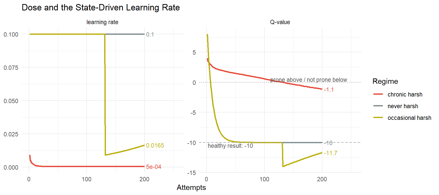
The labels at the end of each line show the settled Q-value (left panel) and the final learning rate (right panel).
Same “kid”, three different “fathers”. The baseline: the patient father’s child lands at $-10$, exactly on the healthy line. The occasional-harsh father’s child tracks the baseline until the first harsh “No”. Each harsh “No” dips the Q-value deep into unhealthy territory, and the suppressed learning rate slows the recovery toward the healthy line; with several shocks spread across the run, she ends the task still below it, her learning rate at a fraction of the baseline. With the chronically harsh father, the frequency of the harsh treatment is so high that the learning rate collapses to its floor and never recovers: the rule is barely learned at all. So, besides the initial big shock, subsequent shocks get diminished, and the kids learn more slowly than in the previous situation. What is interesting here is not only that the state space tracks the learning rate, but that insensitivity to harsh punishment is endogenous to the model.
A new task: harshness carries over
We could test another scenario with the state-space model. Let’s assume the learning rate from one task carries over to a new one. So, once she finishes the 200 attempts learning whether she should climb the chair, she has another learning task. The new task is being nice to your friend. The child starts at $Q_0 = 0$. This means no prior about this behaviour. Every act of kindness the father praises pays $v_{fun}$ = 10. And all fathers are nice here; no shocks. The only difference is the learning rate their harsh history left them with.
simulate_new_task <- function(
    trials = 200,
    phase1 = 200,
    lr0 = 0.1,
    v_fun = 10,
    c_penalty = 20,
    initial_q = 10,
    new_task_q0 = 0,
    harsh_prob = 0.01,
    harsh_severity = 3,
    phi = 0.99,
    beta = 10,
    lr_floor = 0.0005
) {
  h <- 0
  q <- initial_q
  lr <- lr0
  history <- data.frame()
  for (t in 1:(2 * trials)) {
    harsh_event <- ifelse(t <= phase1 & runif(1) < harsh_prob, 1, 0)
    if (t == phase1 + 1) {
      q <- new_task_q0
    }
    if (t <= phase1) {
      reward <- ifelse(harsh_event == 1, v_fun - harsh_severity * c_penalty, v_fun - c_penalty)
    } else {
      reward <- v_fun
    }
    q <- q + lr * (reward - q)
    h <- phi * h + harsh_event
    lr <- max(lr0 / (1 + beta * h), lr_floor)
    history <- rbind(history, data.frame(trial = t, lr = lr, q = q, harsh_event = harsh_event))
  }
  return(history)
}

set.seed(10)
transfer_all <- bind_rows(
  simulate_new_task(harsh_prob = 0.00) %>% mutate(regime = "never harsh"),
  simulate_new_task(harsh_prob = 0.01) %>% mutate(regime = "occasional harsh"),
  simulate_new_task(harsh_prob = 0.60) %>% mutate(regime = "chronic harsh")
)

transfer_final <- transfer_all %>%
  group_by(regime) %>%
  summarise(
    q_old_end = round(q[100], 1),
    q_new_end = round(tail(q, 1), 1),
    lr_new_start = signif(lr[101], 3),
    lr_new_end = signif(tail(lr, 1), 3)
  )
transfer_long <- transfer_all %>%
  pivot_longer(c(q, lr), names_to = "metric", values_to = "value") %>%
  mutate(
    task = factor(ifelse(trial <= 200, "old task", "new task"), levels = c("old task", "new task")),
    trial_in_task = trial - 200 * (trial > 200)
  )
q_panel2 <- transfer_long %>% filter(metric == "q")

ggplot(transfer_long, aes(x = trial_in_task, y = value, color = regime)) +
  geom_line(linewidth = 1) +
  facet_grid(metric ~ task, scales = "free_y", labeller = labeller(
    metric = c(q = "Q-value", lr = "learning rate"),
    task = c("old task" = "old task: climbing is forbidden",
             "new task" = "new task: be nice to your friend")
  )) +
  geom_hline(aes(yintercept = 0), linetype = "dotted", color = "grey60", data = q_panel2) +
  geom_text(data = transfer_long %>% group_by(metric, task, regime) %>% slice_tail(n = 1),
            aes(x = 203, label = ifelse(metric == "q", round(value, 1), signif(value, 3))),
            hjust = 0, size = 3, show.legend = FALSE) +
  scale_x_continuous(limits = c(0, 218)) +
  scale_color_manual(values = c(
    "never harsh" = "#7F8C8D",
    "occasional harsh" = "#BBB111",
    "chronic harsh" = "#E74C3C"
  )) +
  labs(
    title = "A New Task: Only the Learning Rate Carries Over",
    subtitle = "The same 200 attempts, split into the two tasks: the old forbidden rule, then an unrelated task, being nice to your friend, where the father is not harsh and only the learning rate carries over.",
    x = "Attempts in this task",
    y = NULL,
    color = "Regime"
  ) +
  theme_minimal()
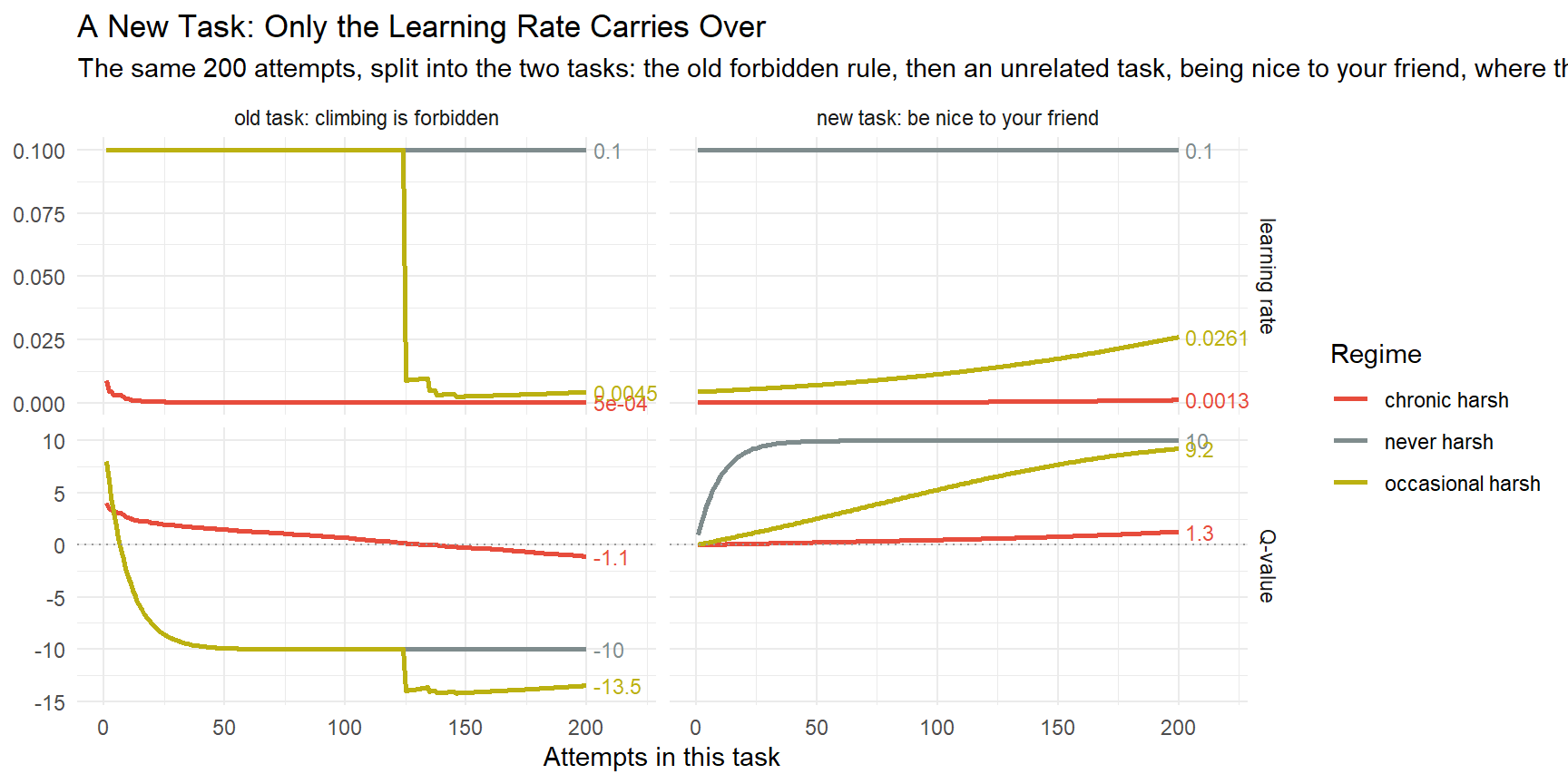
The four facets split the same 200 attempts into the two tasks; the labels at the end of each line show the final Q-value and learning rate per task.
All three children enter the new task with the same $Q_0 = 0$ and make the same kinds of actions. What differs is how quickly they absorb them. As one can see, because of the consequences of the harsh treatment, the occasionally-harsh child, shocked in only 4 of the 200 attempts, still carried the consequences and did not reach the healthy $Q = 10$ threshold. ML readers will recognise this: it is a toy version of loss of plasticity, where an agent’s ability to learn new tasks degrades because of how it learned the old one.
Conclusion
I’ve completed the tasks I set up earlier here. I made a model where: i) caretaker consistency is important and ii) harsh treatment affects learning. As noted earlier, this is a simple model; I doubt that a human brain works exactly like that. But as far as my knowledge goes, this isn’t unconventional: humans need consistency for learning, and teachers and fathers who treat their pupils harshly affect their learning negatively in multiple ways. Next part, I’ll do this exact exercise but using a Bayesian framework.