Can a Baby Learn? Beliefs and Certainty
Part II: Bayesian
Continuing from the last part, let’s now model the kid’s behaviour using a Bayesian approach. Instead of a Q-value updated by prediction error, she now keeps a whole distribution over her belief: not just what she thinks, but how sure she is. She also holds a belief about how much to trust the evidence that shifts that belief.
Here is the same problem: a tempting chair adventure, where a father wants to curb the kid’s willingness. Her belief is about her father: what percentage of the time does he actually say “No” when she tries? She places a Beta prior on $\theta = P(\text{says No})$, started with a small prior strength $K$ (initial stubbornness, prior_strength) and a starting optimism: she believes the father never intervenes, so her desire to climb opens at the full fun value $v_{fun} = 10$. Same starting point as before ($Q_0 = 10$).
with initial_belief = 0 in the climbing task (and a neutral $50/50$ when a new task starts in Section 4, mirroring the companion post’s $Q_0 = 0$ there). Read literally, $\text{Beta}(0, K)$ is not a proper distribution. It is a point belief (“he never says No”) serving as a starting position; the first updates move her off the boundary at once.
Importantly, the child does not take all evidence at face value. The credibility weight $z = \frac{n}{n + K}$ determines how much of an event she takes in. $K$ represents the stubbornness factor; a large $K$ means the kid learns little from the evidence: with $K = 3$, $z$ is still only $0.985$ after two hundred attempts. What saturates quickly is the desire curve, not the weight: her belief is most sensitive when she knows the least, so desire moves fastest at the first trials and flattens asymptotically, close to the curves of the previous part:
$$a \leftarrow a + z \cdot [\text{No}], \qquad b \leftarrow b + z \cdot [\text{Yes}],$$where $[\text{No}]$ is $1$ when the father intervenes on that attempt and $[\text{Yes}]$ is $1$ when he lets her climb. Note that $n$ counts the attempts before the current one, so the very first event arrives at $z = 0$: she needs a moment of history before anything registers.
The desire to climb is the expected payoff under the posterior, with the same targets as before ($v_{fun} = 10$, $c_{penalty} = 20$):
$$\text{desire} = v_{fun} - c_{penalty} \cdot \mathbb{E}[\theta]$$(Section 2 will add a severity factor that multiplies the cost when harshness enters the picture; with no harshness expected it is $1$, so this is the form that matters in this section.)
And because the belief is a distribution, the posterior also carries a second number everywhere: the posterior standard deviation, i.e. how sure the child is. Where the Q-learning child had a step size, this child has a belief and its precision.
library(ggplot2)
library(dplyr)
library(tidyr)

simulate_bayesian_credibility <- function(
    trials = 200,
    phase1 = 200,
    new_task = FALSE,
    prior_strength = 3,
    initial_belief = 0,
    new_task_belief = 0.5,
    new_task_prior_strength = 10,
    harsh_weight = 7,
    no_prob = 1,
    harsh_prob = 0,
    harsh_severity = 3,
    stubbornness_growth = 50,
    v_fun = 10,
    c_penalty = 20,
    kappa_a0 = 0.1,
    kappa_b0 = 9.9
) {
  K <- prior_strength
  harsh_seen <- 0
  history <- data.frame()
  for (t in 1:(if (new_task) 2 * trials else trials)) {
    if (t == 1) {
      a <- initial_belief * prior_strength
      b <- (1 - initial_belief) * prior_strength
      ca <- kappa_a0
      cb <- kappa_b0
    }
    if (new_task && t == phase1 + 1) {
      a <- new_task_belief * new_task_prior_strength
      b <- (1 - new_task_belief) * new_task_prior_strength
      ca <- kappa_a0
      cb <- kappa_b0
    }
    if (t <= phase1) {
      intervene <- ifelse(runif(1) < no_prob, 1, 0)
      harsh_event <- ifelse(intervene == 1 & runif(1) < harsh_prob, 1, 0)
      z <- (t - 1) / (t - 1 + K)
      if (harsh_event == 1) {
        a <- a + z
        ca <- ca + harsh_weight * z * z
        harsh_seen <- harsh_seen + 1
      } else if (intervene == 1) {
        a <- a + z
        cb <- cb + z
      } else {
        b <- b + z
      }
      K <- prior_strength + stubbornness_growth * harsh_seen
      theta <- a / (a + b)
      kappa <- ca / (ca + cb)
      sd <- sqrt(a * b / ((a + b)^2 * (a + b + 1)))
      desire <- v_fun - c_penalty * theta * (1 + (harsh_severity - 1) * kappa)
      z2 <- NA
    } else if (new_task) {
      z2 <- (t - phase1 - 1) / (t - phase1 - 1 + K)
      b <- b + z2
      theta <- a / (a + b)
      kappa <- NA
      sd <- sqrt(max(a, 1) * b / ((a + b)^2 * (a + b + 1)))
      desire <- v_fun - c_penalty * theta
    }
    history <- rbind(history, data.frame(
      trial = t, theta = theta, sd = sd, desire = desire,
      kappa = kappa, harsh = harsh_seen,
      z = ifelse(is.na(z2), (t - 1) / (t - 1 + K), z2)
    ))
  }
  return(history)
}
1. Consistent vs. Inconsistent Father
Same as in part one, we have two fathers: one that says “No” every time and another that says “No” $70\%$ of the time. The kids also have 200 attempts each.
set.seed(101)
consistent <- simulate_bayesian_credibility(trials = 200, phase1 = 200, no_prob = 1, harsh_prob = 0)
inconsistent <- simulate_bayesian_credibility(trials = 200, phase1 = 200, no_prob = 0.7, harsh_prob = 0)

belief_data <- bind_rows(
  consistent %>% mutate(regime = "consistent (100% No)"),
  inconsistent %>% mutate(regime = "inconsistent (70% No)")
) %>%
  mutate(
    desire_lo = 10 - 20 * (theta + 1.96 * sd),
    desire_hi = 10 - 20 * (theta - 1.96 * sd)
  )
ggplot(belief_data, aes(x = trial, y = desire, color = regime)) +
  geom_ribbon(aes(ymin = desire_lo, ymax = desire_hi, fill = regime, group = regime), alpha = 0.12, color = NA) +
  geom_line(linewidth = 1) +
  geom_hline(yintercept = -10, linetype = "dashed", color = "grey60") +
  geom_hline(yintercept = 0, linetype = "dotted", color = "grey60") +
  annotate("text", x = 2, y = -10.9, label = "healthy result: -10", hjust = 0, color = "grey35", size = 3) +
  annotate("text", x = 190, y = 0.5, label = "prone above / not prone below", hjust = 1, color = "grey35", size = 3) +
  geom_text(data = belief_data %>% group_by(regime) %>% slice_tail(n = 1),
            aes(x = 203, label = round(desire, 1)), hjust = 0, size = 3.2, show.legend = FALSE) +
  scale_x_continuous(limits = c(0, 218)) +
  scale_y_continuous(limits = c(-13, 19)) +
  scale_color_manual(values = c(
    "consistent (100% No)" = "#2E86AB",
    "inconsistent (70% No)" = "#A23B72"
  )) +
  scale_fill_manual(values = c(
    "consistent (100% No)" = "#2E86AB",
    "inconsistent (70% No)" = "#A23B72"
  )) +
  labs(
    title = "Consistent vs. Inconsistent Feedback: Belief and Credible Band",
    subtitle = "Lines are the expected desire under the posterior; bands are +/- 1.96 posterior SDs.",
    x = "Number of Attempts",
    y = "Desire to Climb (Expected Payoff)",
    color = "Father",
    fill = "Father"
  ) +
  theme_minimal()
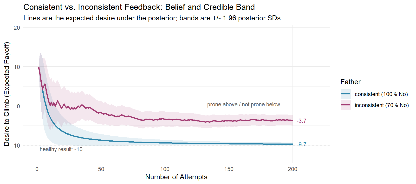
The labels at the end of each line show the settled desire.
Both children learn the right point: the consistent kid’s belief converges towards the always-“No” father. This means the desire converges to -9.7, slightly off the “healthy no” line of $-10$. This happens because of the finite credibility weight; the belief approaches certainty in the limit, never quite arriving (after 200 tries her $\theta$ sits at 0.984). The inconsistent kid’s belief approaches the true $70\%$ (her $\theta$ sits at 0.683), and her desire lands on -3.7, finishing close to $-4$, same as the previous text.
Note the band. The consistent child’s posterior shrinks to ±0.02 (sd = 0.00903); the inconsistent child’s band settles about 3.7 times wider, ±0.07 (sd = 0.0337), so she never gets a clean read on her father. The Q-learning child in the companion post wobbled because the signal was noise. The Bayesian child’s line is smoother, but her uncertainty tells the same story: an inconsistent father keeps the kid from fully internalizing the lesson.
2. Adding Harsh Punishment
Now the father always intervenes, but rarely, with probability $\varepsilon = 0.01$, the “No” is harsh, at $s = 3$ times the cost. The child holds a second small belief: what fraction of “No"s are the harsh kind, $\kappa \sim \text{Beta}(c_a, c_b)$, starting near zero. Every plain “No” adds a small count to $c_b$; a harsh “No” is counted harsh_weight = 7 times harder than a plain one, but it arrives through the same credibility filter, so its effective weight is harsh_weight · z². (A harsh “No” also counts as a regular “No” for $\theta$.) The harsh event must pass two gates: it registers only at the credibility volume $z$, and its severity is counted through the same trust: the $7\times$ attention bonus amplifies admitted evidence, not raw events:
The expected payoff is then
$$\text{desire} = v_{fun} - c_{penalty} \cdot \mathbb{E}[\theta] \cdot \big(1 + (s - 1)\, \mathbb{E}[\kappa]\big).$$Why $1 + (s-1)\,\kappa$?
The child holds two beliefs: $\theta = P(\text{the father intervenes})$ and $\kappa = P(\text{harsh} \mid \text{intervenes})$. The expected payoff is:
Outcome Probability (P(Outcome)) Payoff (r) (a) No intervention $1 - \theta$ $v_{fun}$ (b) Plain “No” $\theta\,(1 - \kappa)$ $v_{fun} - c_{penalty}$ (c) Harsh “No” $\theta\,\kappa$ $v_{fun} - s\,c_{penalty}\ \ (s = 3)$ Expected payoff:
$$\mathbb{E}[r] = P(a) \cdot r_a + P(b) \cdot r_b + P(c) \cdot r_c$$$$\mathbb{E}[r] = (1-\theta)\,v_f + \theta(1-\kappa)(v_f - c) + \theta\kappa\,(v_f - s\,c)$$The $v_f$ terms:
$$(1-\theta)v_f + \theta(1-\kappa)v_f + \theta\kappa v_f = v_f$$What’s left is the expected cost, and the key is factoring it:
$$\text{cost} = \theta(1-\kappa)\,c + \theta\kappa\,s\,c = \theta\,c\,[(1-\kappa) + s\kappa] = \theta\,c\,[1 + (s-1)\kappa]$$So the formula is just:
$$\mathbb{E}[r] = v_f - c\,\theta\,\big(1 + (s-1)\,\kappa\big)$$Also, note that $\mathbb{E}[\theta] \cdot \big(1 + (s - 1)\, \mathbb{E}[\kappa]\big)$ is the exact form under one assumption: we treat the two posterior beliefs as independent, because $\theta$ and $\kappa$ are updated in separate parameter pairs ($a$/$b$ vs $c_a$/$c_b$), so $\mathbb{E}[\theta \cdot \kappa] = \mathbb{E}[\theta] \cdot \mathbb{E}[\kappa]$. Strictly speaking, the two beliefs share the same evidence stream (a harsh “No” moves both), so the independence is a simplification, and a harmless one at these effect sizes.
A modeling note: the $z^2$ filter is a choice. It encodes “stops listening”: when trust collapses, the severity evidence collapses with it. The alternative, a single gate with $7 \cdot z$ and no second trust discount, keeps a hypervigilant channel: the shocked child keeps registering harshness even when she stops trusting, and in the chronic scenario her desire ends deep in the fear zone, about -23.1. We chose the two gates; a hypervigilant child is a different model.
set.seed(101)
harsh_data <- bind_rows(
  simulate_bayesian_credibility(trials = 200, phase1 = 200, harsh_prob = 0.00) %>% mutate(regime = "never harsh"),
  simulate_bayesian_credibility(trials = 200, phase1 = 200, harsh_prob = 0.01) %>% mutate(regime = "occasional harsh")
) %>%
  mutate(
    desire_lo = 10 - 20 * (theta + 1.96 * sd) * (1 + 2 * kappa),
    desire_hi = 10 - 20 * (theta - 1.96 * sd) * (1 + 2 * kappa)
  )

occ_desire <- harsh_data$desire[harsh_data$regime == "occasional harsh"]
occ_shocks <- which(diff(c(0, harsh_data$z[harsh_data$regime == "occasional harsh"])) < -0.05)
occ_steps <- round(occ_desire[occ_shocks] - occ_desire[occ_shocks - 1], 1)
ggplot(harsh_data, aes(x = trial, y = desire, color = regime)) +
  geom_ribbon(aes(ymin = desire_lo, ymax = desire_hi, fill = regime, group = regime), alpha = 0.12, color = NA) +
  geom_line(linewidth = 1) +
  geom_hline(yintercept = -10, linetype = "dashed", color = "grey60") +
  geom_hline(yintercept = 0, linetype = "dotted", color = "grey60") +
  annotate("text", x = 2, y = -10.9, label = "healthy result: -10", hjust = 0, color = "grey35", size = 3) +
  annotate("text", x = 190, y = 0.5, label = "prone above / not prone below", hjust = 1, color = "grey35", size = 3) +
  geom_text(data = harsh_data %>% group_by(regime) %>% slice_tail(n = 1),
            aes(x = 203, label = round(desire, 1)), hjust = 0, size = 3.2, show.legend = FALSE) +
  scale_x_continuous(limits = c(0, 218)) +
  scale_y_continuous(limits = c(-16, 19)) +
  scale_color_manual(values = c(
    "never harsh" = "#7F8C8D",
    "occasional harsh" = "#BBB111"
  )) +
  scale_fill_manual(values = c(
    "never harsh" = "#7F8C8D",
    "occasional harsh" = "#BBB111"
  )) +
  labs(
    title = "A Harsh No Is Priced Forever",
    subtitle = "Rare harsh events step the desire down permanently: she updates her belief about severity, and never hears the correction.",
    x = "Attempts",
    y = "Desire to Climb (Expected Payoff)",
    color = "Regime",
    fill = "Regime"
  ) +
  theme_minimal()
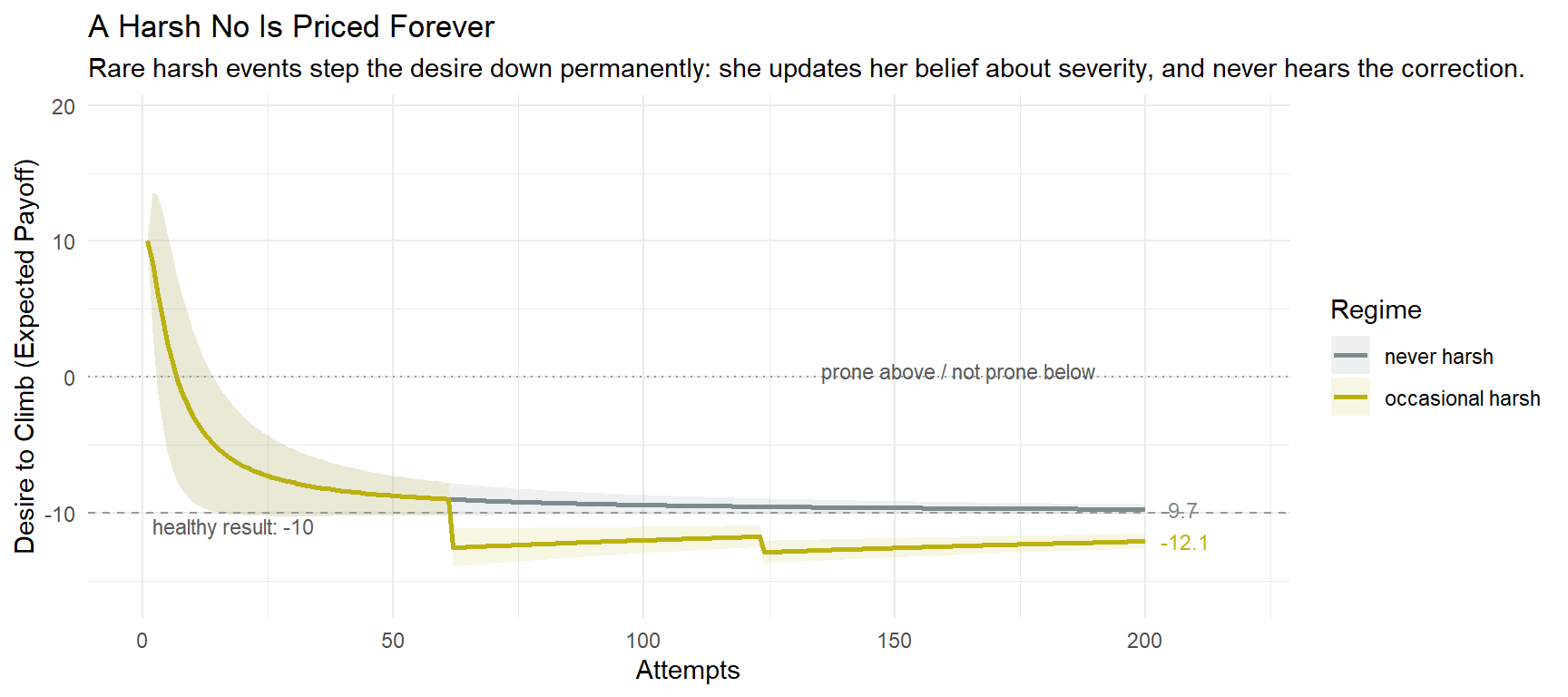
The labels at the end of each line show the settled desire.
The rare harsh event is surprising evidence: a harsh “No” is heard at harsh_weight = 7 times the weight of a plain one, through the same credibility filter (harsh_weight · z²), so it moves the severity belief hard. This is the Bayesian fingerprint: the step it causes never recovers. The first shock alone costs -3.6 points, about half of Part I’s early shock, where one harsh “No” dropped the Q-value by roughly $4$ points in a single update; the second costs -1.1. By the end the occasional-harsh child sits at -12.1 while the never-harsh child sits at -9.7. One harsh “No” in a hundred changes the whole expected payoff: harshness is cheap to have, and hard to un-have.
3. Chronic Harshness: The Child Who Stops Trusting
The dose increases. The state-space view of the companion post hid a harshness state that suppressed the step size. Here harshness attacks the other lever: every harsh event makes the child more stubborn, and the credibility weight’s $K$ grows with each shock (stubbornness_growth = 50), so the evidence arrives at a smaller and smaller volume:
set.seed(101)
bayesian_all <- bind_rows(
  simulate_bayesian_credibility(harsh_prob = 0.00) %>% mutate(regime = "never harsh"),
  simulate_bayesian_credibility(harsh_prob = 0.01) %>% mutate(regime = "occasional harsh"),
  simulate_bayesian_credibility(harsh_prob = 0.60) %>% mutate(regime = "chronic harsh")
) %>%
  mutate(
    desire_lo = 10 - 20 * (theta + 1.96 * sd) * (1 + 2 * kappa),
    desire_hi = 10 - 20 * (theta - 1.96 * sd) * (1 + 2 * kappa)
  )

bayesian_long <- bayesian_all %>%
  pivot_longer(c(desire, sd), names_to = "metric", values_to = "value") %>%
  mutate(metric = factor(metric, levels = c("desire", "sd")))

bayesian_final <- bayesian_all %>%
  group_by(regime) %>%
  summarise(
    desire_end = round(tail(desire, 1), 1),
    sd_end = signif(tail(sd, 1), 3),
    z_end = signif(tail(z, 1), 3),
    kappa_end = signif(tail(kappa, 1), 3),
    theta_end = round(tail(theta, 1), 3),
    shocks = max(harsh)
  )
desire_panel <- bayesian_long %>% filter(metric == "desire")
sd_panel <- bayesian_long %>% filter(metric == "sd")

ggplot(bayesian_long, aes(x = trial, y = value, color = regime)) +
  geom_ribbon(aes(ymin = desire_lo, ymax = desire_hi, fill = regime, group = regime),
              alpha = 0.12, color = NA, data = desire_panel) +
  geom_line(linewidth = 1) +
  facet_wrap(~metric, scales = "free_y", labeller = as_labeller(c(desire = "desire to climb", sd = "posterior uncertainty (SD of theta)"))) +
  geom_hline(aes(yintercept = -10), linetype = "dashed", color = "grey60", data = desire_panel) +
  geom_hline(aes(yintercept = 0), linetype = "dotted", color = "grey60", data = desire_panel) +
  geom_text(data = desire_panel, aes(x = 2, y = -10.9, label = "healthy result: -10"), hjust = 0, color = "grey35", size = 3) +
  geom_text(data = bayesian_long %>% group_by(metric, regime) %>% slice_tail(n = 1),
            aes(x = 203, label = ifelse(metric == "desire", round(value, 1), signif(value, 3))),
            hjust = 0, size = 3, show.legend = FALSE) +
  scale_x_continuous(limits = c(0, 218)) +
  scale_color_manual(values = c(
    "never harsh" = "#7F8C8D",
    "occasional harsh" = "#BBB111",
    "chronic harsh" = "#E74C3C"
  )) +
  scale_fill_manual(values = c(
    "never harsh" = "#7F8C8D",
    "occasional harsh" = "#BBB111",
    "chronic harsh" = "#E74C3C"
  )) +
  labs(
    title = "Chronic Harshness: Dose and the Credibility Weight",
    subtitle = "Each harsh event grows the stubbornness K, so the evidence arrives at a smaller volume. Left: expected desire with 95% credible band. Right: posterior SD.",
    x = "Attempts",
    y = NULL,
    color = "Regime",
    fill = "Regime"
  ) +
  theme_minimal()
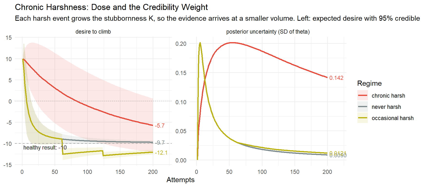
The labels at the end of each line show the settled desire (left) and the final posterior SD (right).
The never-harsh child ends at -9.7, the occasional-harsh child at -12.1. The chronic-harsh child ends at -5.7, partway to the healthy -10. Harshness arrives through the same credibility filter as everything else (harsh_weight · z²), so once her trust collapsed the severity evidence stopped landing too: her severity belief sits at 0.0698, hardly higher than the occasional child’s, and her $\theta$ is stuck at 0.69. She carries the widest uncertainty of the three: posterior SD 0.142 (the never-harsh child’s is 0.00903), a 95% band wider than the space between the two reference lines. Her credibility weight collapsed to 0.0349: after 110 shocks she hears roughly three percent of the evidence that reaches other children. The child who has been shocked the most is the child who believes the world the least: she half-learned the rule, and she knows she doesn’t know it. The Q-learning child froze because her step size collapsed; the Bayesian child freezes because her trust did.
4. A New Task: Only the Trust Carries Over
Now the same question as before: what happens to the next thing the child tries to learn? The companion post’s answer was that only the learning rate carried over. The Bayesian answer is symmetric: the belief itself resets, and a new context (“be nice to your friend”) means a fresh $50/50$ prior, though a stronger one than she was born with (new_task_prior_strength = 10 against the original $3$), so the desire starts at $0$, exactly where the companion post’s child started her new task. Because the old task taught the child nothing about being kind, what carries over is the trust: the stubbornness $K$ accumulated in the old task. The kind acts pay $v_{fun} = 10$, the father is not harsh here, and the three children see exactly the same two hundred kind acts; nothing is random in this task, so the evidence is identical for all three.
set.seed(101)
transfer_all <- bind_rows(
  simulate_bayesian_credibility(harsh_prob = 0.00, new_task = TRUE) %>% mutate(regime = "never harsh"),
  simulate_bayesian_credibility(harsh_prob = 0.01, new_task = TRUE) %>% mutate(regime = "occasional harsh"),
  simulate_bayesian_credibility(harsh_prob = 0.60, new_task = TRUE) %>% mutate(regime = "chronic harsh")
) %>%
  mutate(
    desire_lo = ifelse(trial <= 200,
                       10 - 20 * (theta + 1.96 * sd) * (1 + 2 * kappa),
                       10 - 20 * (theta + 1.96 * sd)),
    desire_hi = ifelse(trial <= 200,
                       10 - 20 * (theta - 1.96 * sd) * (1 + 2 * kappa),
                       10 - 20 * (theta - 1.96 * sd))
  )

transfer_long <- transfer_all %>%
  pivot_longer(c(desire, sd), names_to = "metric", values_to = "value") %>%
  mutate(
    metric = factor(metric, levels = c("desire", "sd")),
    task = factor(ifelse(trial <= 200, "old task", "new task"), levels = c("old task", "new task")),
    trial_in_task = trial - 200 * (trial > 200)
  )

transfer_final <- transfer_all %>%
  group_by(regime) %>%
  summarise(
    desire_new_end = round(tail(desire, 1), 1),
    sd_new_end = signif(tail(sd, 1), 3),
    theta_new_end = round(tail(theta, 1), 3),
    z_new = signif(tail(z, 1), 3),
    shocks = max(harsh),
    time_to_7 = suppressWarnings(min(which(desire[201:400] >= 7)))
  )
desire_panel2 <- transfer_long %>% filter(metric == "desire")

ggplot(transfer_long, aes(x = trial_in_task, y = value, color = regime)) +
  geom_ribbon(aes(ymin = desire_lo, ymax = desire_hi, fill = regime, group = regime),
              alpha = 0.12, color = NA, data = desire_panel2) +
  geom_line(linewidth = 1) +
  facet_grid(metric ~ task, scales = "free_y", labeller = labeller(
    metric = c(desire = "desire (expected payoff)", sd = "posterior uncertainty (SD)"),
    task = c("old task" = "old task: climbing is forbidden",
             "new task" = "new task: be nice to your friend")
  )) +
  geom_hline(aes(yintercept = 0), linetype = "dotted", color = "grey60", data = desire_panel2) +
  geom_hline(aes(yintercept = -10), linetype = "dashed", color = "grey60", data = desire_panel2 %>% filter(task == "old task")) +
  geom_text(data = desire_panel2 %>% filter(task == "old task"), aes(x = 2, y = -11.2, label = "healthy result: -10"), hjust = 0, color = "grey35", size = 2.6) +
  geom_text(data = transfer_long %>% group_by(metric, task, regime) %>% slice_tail(n = 1),
            aes(x = 203, label = ifelse(metric == "desire", round(value, 1), signif(value, 3))),
            hjust = 0, size = 3, show.legend = FALSE) +
  scale_x_continuous(limits = c(0, 218)) +
  scale_color_manual(values = c(
    "never harsh" = "#7F8C8D",
    "occasional harsh" = "#BBB111",
    "chronic harsh" = "#E74C3C"
  )) +
  scale_fill_manual(values = c(
    "never harsh" = "#7F8C8D",
    "occasional harsh" = "#BBB111",
    "chronic harsh" = "#E74C3C"
  )) +
  labs(
    title = "A New Task: Only the Trust Carries Over",
    subtitle = "The belief resets to 50/50 in the new task; the stubbornness K does not. Ribbons are 95% posterior bands.",
    x = "Attempts in this task",
    y = NULL,
    color = "Regime",
    fill = "Regime"
  ) +
  theme_minimal()
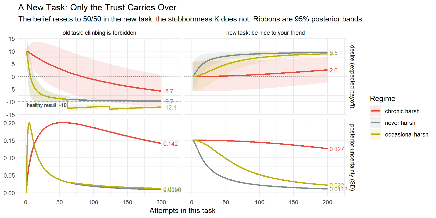
The four facets split the same 400 attempts into the two tasks; labels show the final desire and posterior SD per task.
The never-harsh child enters with $K = 3$ and hears the kind acts at volume 0.985: she is past a desire of $+7$ by her 32-th attempt and ends at 9.5. The occasional-harsh child carries $K$ from her two shocks (volume 0.659) and ends at 9, with a posterior SD of 0.022 instead of 0.0112: she learns, but always a step behind, and never as sure.
The chronic-harsh child carries $K$ from 110 shocks into the new task and hears the kindness at volume 0.0349, about three percent. After two hundred kind acts her belief about being punished has moved from $0.5$ to 0.37 (the never-harsh child’s fell to 0.025), and her desire ends at 2.6, not far from where every child started. Her uncertainty, 0.127, remains the widest of the three, because she could not let the evidence in.
That is the Bayesian version of the same punchline: treatment harsh enough to break trust does not just fail to teach the old rule, it makes the next rule unteachable. The two children agree on the outcome, and disagree on the mechanism. The Q-learning child stops because her updates are too small; the Bayesian child stops because her beliefs are too stubborn. One stops updating; the other stops listening.
Conclusion
Part I promised this same exercise in a Bayesian framework, and the outcome is unchanged: consistency teaches, a rare harsh “No” is priced forever, and chronic harshness breaks the learner. What the Bayesian lens adds is where the damage lands. A shock that never repeats still moves the severity belief, and nothing in a consistent future will ever correct it. A shock that keeps repeating moves something deeper: the credibility weight itself, and with it the child’s ability to hear the next lesson at all. The Q-learning child’s step size collapsed; the Bayesian child’s trust did.
As in Part I, this is a toy model: no child runs Beta updates in her head. But when two very different learning rules land on the same three lessons about consistency and harshness, I trust the lessons more than either model.